Creating Motion Profile Tables
A motion profile table is a table of unit-less position values, which are the integral of the velocity profile during the acceleration and deceleration process of a motion task. A motion profile can be stored in the drive and used in order to accelerate and decelerate with a certain profile shape.
The motion profile table describes the shape of the acceleration process, but does not determine how fast the motion task accelerates or decelerates and which target velocity will be reached.
Example of a motion profile table
An example of a motion profile table is shown below:
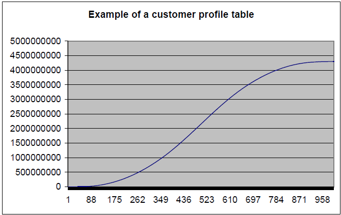
The motion profile table is the integral of the velocity profile. The velocity profile during the acceleration and the deceleration process is shown below:
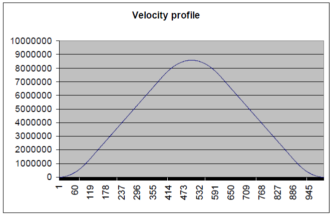
The derivative of the motion profile table is calculated using the following formula:
velocity_profile_valuen = customer_profile_entryn+1 - customer_profile_entryn
Motion Profile Table Restrictions
Restrictions for motion profile tables include the following:
- A motion profile table needs a reasonable number of entries (usually between 1,000-4,000 entries, depending on the acceleration and deceleration time of a motion task). If an acceleration or deceleration process takes more position-loop samples than half of the motion profile table entries, then the drive interpolates linearly between the single motion profile table entries.
- The motion profile table should contain an even number of entries. The first point of the customer table starts with the value of 0 and the last point must contain the value of 232-1.
- The motion profile table contains values in ascending order.
- The following motion profile table entry must contain the value of nearly 231.
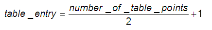
Example
Assume that a motion profile table contains 1,000 data points. In this case point 1000/2+1 = 501 must contain the value of 231 = 2,147,483,648.
- A motion profile table must also be symmetric during the acceleration and the deceleration process when Profile Table interpolation is used.
To illustrate profile symmetry, the derivative of the motion profile table (velocity profile) is shown below. Note the symmetry according to the velocity profile.
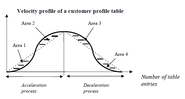
The left half of the curve describes the shape of the acceleration process of the motion task. The right half of the curve describes the shape of the deceleration process of the motion task. A symmetric motion profile table means that Area 1, Area 2, Area 3 and Area 4 have the same size.
Different methods of motion table motion tasking
General motion profile table explanations
The algorithm for handling the motion profile motion task are the same for both methods, the standard customer table motion task and the OneToOne customer table motion task. The diagram below illustrates a basic table profile algorithm. The figure shows a standard customer table motion task.
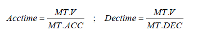
The drive calculates the acceleration time and deceleration time out of the given motion task parameters (see MT Parameters and Commands) with the assumption of a trapezoidal acceleration setting (MT.ACC and MT.DEC). The formulas are:
Use of IL.KACCFF with Motion Tables
IL![]() "Instruction list"
This is a low-level language and resembles assembly.KACCFF can be used with Profile Table or OneToOne interpolation motion tasks as long as the following criteria is met:
"Instruction list"
This is a low-level language and resembles assembly.KACCFF can be used with Profile Table or OneToOne interpolation motion tasks as long as the following criteria is met:
(Acctime + Dectime) < (number_of_table_points/4000)
If this criteria is not met, a current spikes at 4KHz will occur.
Profile Table Interpolation Motion Task
The Profile Table interpolation motion task is displayed in the following figure:
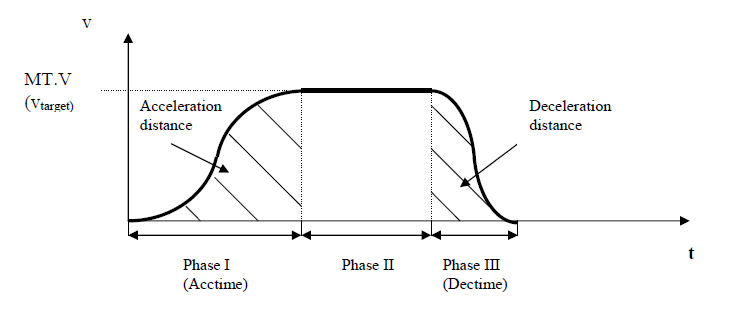
The Profile Table interpolation for a stand-alone motion task (the motion task does not automatically trigger a following motion task) can be separated in three different phases:
- Phase I: The drive steps within a pre-calculated acceleration time through the first half of the motion profile table and reaches finally the requested target velocity of the motion task.
- Phase II: The drive inserts a constant velocity phase and checks continuously if a brake-point has been crossed. The brake-point is naturally the target position minus the deceleration distance.
- Phase III: The drive steps into the second half of the motion profile table and reaches finally the requested target position when the velocity becomes zero. The step into the second half of the motion profile table is a critical point and requires a symmetric table and the value of 231 at entry number_of_table_points / 2 + 1 as explained in Motion Profile Table Restrictions for a customer table.
OneToOne interpolation motion task
The OneToOne interpolation motion task is basically very similar to the Profile Table interpolation motion task handling with just a few small differences.
- The OneToOne customer table motion task does not step out of the table after an acceleration process and inserts a constant profile (Phase II in the section above). The OneToOne handling steps within a pre-calculated time through the whole table in one go and cover the required distance.
- A change-on-the-fly from one motion task to another without finishing the first motion task is not possible for this mode.
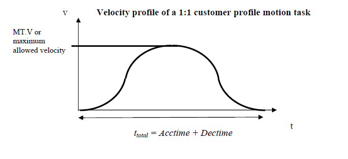
- The OneToOne profile does not use different acceleration and deceleration values. The AKD calculates the sum of the acceleration time and deceleration time and uses this total time (total¬= MT.V/DRV.ACC+MT.V/MT.DEC) for the motion task as explained in the following picture. In case that the acceleration + deceleration time is too small for moving a certain distance, which would lead into a too large peak-velocity, the total time will automatically be extended to the required value in order to not exceed the maximum allowed velocity to the minimum of MT.V or VL.LIMITP and VL.LIMITN.
Note that the motion task target velocity is only reached in case of a symmetric table. The velocity will be different when the profile table is non-symmetric.
Setting up a motion profile motion task
It is also possible to select to adjust a motion task on a command line level with the help of the MT commands. There are 2 commands which are mentioned within this chapter:
- Trapezoidal, OneToOne, or Profile Table moves are selected using bits 10 and 11 of the MT.CNTL command.
- The MT.TNUM selects which of the 8 tables (0 to 7) to use for the profile. The parameter MT.TNUM will be ignored in the case that a trapezoidal motion task has been selected.
Drive reaction on impossible motion tasks
For all motion tasks, which use a motion profile table as the shape for the velocity profile, the motion task properties must be pre-calculated and it must be evaluated in advance, if a motion task can be handled without any problems or if some of the motion task parameters must be re-calculated automatically by the AKD.
An impossible motion task occurs when the user has not specified enough movement in order to accelerate to the motion task target velocity and to decelerate to velocity 0 without exceeding the distance to travel.
OneToOne interpolation limitations
A OneToOne interpolation motion task cannot be activated while another motion-task isrunning. A OneToOne interpolation motion task must start from velocity 0.
When using a OneToOne interpolation motion task the AKD pre-calculates the expected peak-velocity and checks if the velocity exceeds the minimum of the MT.V, VL.LIMITP and VL.LIMITN .
The expected peak-velocity according to the figure above can be calculated via using the following formula:
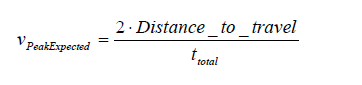
The ‘distance to travel’ is defined in the motion task settings MT.P and MT.CNTL. In case that VPeakExpected exceeds the minimum of the MT.V, VL.LIMITP or VL.LIMITN setting, the AKD re-calculates the total so that VPeakExpected does not exceed the velocity limitations.
The AKD accelerates and decelerates within the same time in case of a OneToOne profile and therefore different settings for MT.ACC and MT.DEC are not considered.
Profile Table interpolation limitations
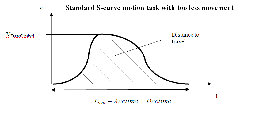
Starting from velocity 0 without change-on-the-fly to a following motion task
If there is not enough ‘distance to travel’ selected by the user in order to accelerate to the target velocity via the selected acceleration (internally converted to acceleration time) and deceleration (internally converted to deceleration time), the AKD lowers the target velocity automatically to VTargetLimited and accelerates within the selected acceleration time to the limited target velocity and decelerates afterward with the selected deceleration time to velocity 0.
The shape of the velocity profile will look like the following pictures with the assumption, that MT.ACC and MT.DEC have different values.
During a change on the fly condition
There are 2 different kinds of considerations within the AKD firmware for a change-on-the-fly condition.
- A change on the fly in the same direction (the target velocity of the previous and the following motion task have the same algebraic sign).
- A change on the fly in the opposite direction (the target velocity of the previous and the following motion task have a different algebraic sign).
Since the shape of a customer table is unknown to the AKD, the drive verifies in advance the validity of the motion task with the assumption of a symmetric motion profile table.
Movement to the same direction
The following figure displays a movement in the same direction, in this case in a positive direction.
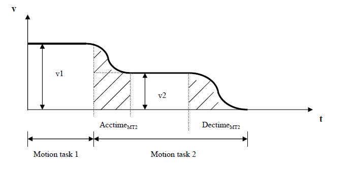
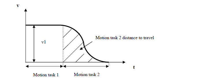
In case that the distance to the target position of the motion task 2 is smaller than distmin, the AKD generates a profile as shown in the next figure.
Movement in different directions
The switch on the fly from a positive velocity to a negative velocity is described in the next figure.
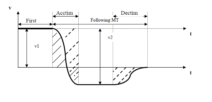
It is not possible to pre-calculate exactly the area, which is marked with solid lines of the following motion task since the shape of the motion profile table is unknown to the drive. This means that it is not possible to identify the movement in positive and negative direction during a change on the fly from v1 to v2. A criterion that a change on the fly will be executed by the drive is, if the total movement in negative direction of the following MT is larger than the area, which is marked with dashed lines. In this case it is ensured, that there will be definitely enough total movement of the MT in negative direction, because the motor moves during the acceleration from v1 to v2 also a bit in positive direction. The magnitude of v2 is in this case the ‘target velocity of MT1’ + ‘target velocity of MT2.'
The drive behaves as follows in case that the hatched area is smaller than the distance to travel
negative direction:
- The drives stops the first motion task with the assigned deceleration ramp.
- Afterwards the following motion task is triggered automatically by the drive starting from velocity 0.


